The conic sections are a family of shapes consisting of parabolas, hyperbolas, and ellipses. Conic sections show up in many scientific applications; for example, celestial orbits trace out different conic sections depending on their energy[1]. The shadow cast by a sundial's "spike" (gnomon) traces out a different conic section depending on latitude and time of year[2]. And mirrors shaped like conic sections have important optical properties for focusing light[3].
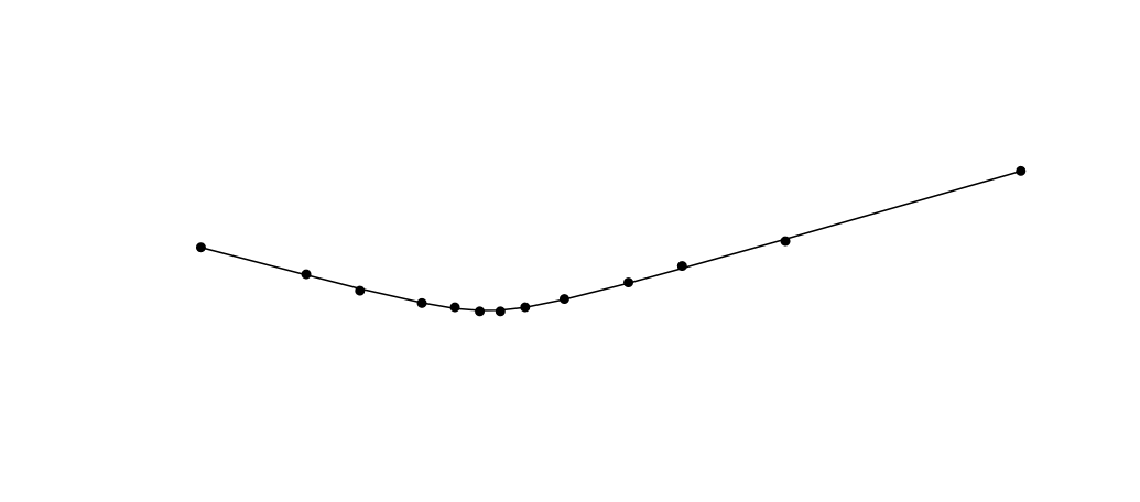
It's therefore useful to be able to take some imprecise physical measurements and fit a conic-shaped curve to them. In this article, I provide some code for doing this. The figure above illustrates fitting some real data points for a sundial; the algorithm finds the hyperbolic shape shown.
Algebraically, conic sections are the graphs of the equation: $$Ax^2 + Bxy + Cy^2 + Dx + Ey + F = 0$$
(It's just any general polynomial you can make involving x and y where no term has a combined exponent bigger than two.) There is some beautiful linear algebra under the hood; one useful fact is that the discriminant \(B^2-4AC\) is either positive, negative, or zero, which tells you whether the shape is an ellipse, hyperbola, or parabola.
To measure how well a particular conic section fits your data \(\langle
x_i, y_i\rangle\), you might imagine a straightforward algorithm: compute \(A x_i^2 + Bx_iy_i + C y_i^2 + D x_i + E y_i + F\) for each data point, square those values and add them up, then see how far away the sum is from zero. To find the optimal fit, vary the coefficients to make this sum as close to zero as possible.
This basic approach almost works, despite the search space being unstable[4]. You can modify it to make it more stable and to allow the user to specify a target conic type (hyperbola, parabola, or ellipse) in advance. In a paper by Nievergelt, the author describes how to do this. I implemented the suggested algorithm in Python, as shown below.
Interestingly, the algorithm gets less stable the better the data fit a particular conic; a little empirical noise is useful. Because my target application (determining whether a blackbox function represents a conic) involved extremely accurate conic sections, this threw off my results. So I modified the algorithm slightly. Where the algorithm uses an SVD decomposition to decide whether the points all lie on a line, I use the Theil-Sen estimator[5].
I also found a few typos in the manuscript, which when fixed allowed me to exactly reproduce the curves in the paper.
In a flyby, the object has enough surplus energy to escape the gravitational pull, and gets flung out along a hyperbolic orbit. In a closed orbit, the object remains gravitationally captive, tracing an elliptic orbit. In the parabolic case, the object has just enough energy to exactly cancel the gravitational pull, and also escapes. ↩︎
For most places, the sun rises and sets, spending the night below the horizon. In this case, the gnomon's shadow traces out a hyperbolic path over the course of the day. Near the poles, the sun might spend the entire day above the horizon, and the shadow traces out an ellipse. In the exact intermediate case, the sun barely grazes the horizon before rising again, and the shadow traces out a parabola. ↩︎
See the Cassegrain telescope design, for example. ↩︎
Small variations in data can cause large variations in best-fit conic; infinitesimal changes to a parabola will make it an ellipse or hyperbola; the algorithm can often fit non-conic data extremely closely, which is unfortunate for detecting conics. ↩︎
The Theil-Sen estimator is a neat simple algorithm to find a best-fit line to some data: First, you compute all lines through all pairs of points. Then you determine the median slope \(m\) among the slopes of those lines. Second, you draw a line of slope \(m\) through each of the data points and compute their y-intercepts. Find the median intercept value \(b\). The overall fit line is \(y=mx+b\), and it's particularly resistant to outliers because we used medians throughout. ↩︎
Source code
from numpy.linalg import svd, qr, solve, det
from numpy import array, matmul, float64, transpose # , allclose, matmul, float64
from math import sqrt

#### Given a list of 2D points, return an array
#### describing the best-fit conic. Returns something special in the
#### case of degenerate conics (e.g. straight lines)

# See paper: Yves Nievergelt, "Fitting conics of specific types to
# data"


SMALL = 10**-12
sqrt2 = 2**0.5

TYPE_HYPERBOLA = "hyperbola"
TYPE_PARABOLA = "parabola"
TYPE_ELLIPSE = "ellipse"


def centered(points) :
    """Subtract the average from the (x,y) pairs."""
    xs_uncentered = [x for (x,y) in points]
    ys_uncentered = [y for (x,y) in points]

    x_center = sum([x for x in xs_uncentered])/len(points)
    y_center = sum([y for y in ys_uncentered])/len(points)

    xs = [x-x_center for x in xs_uncentered]
    ys = [y-y_center for y in ys_uncentered]

    return list(zip(xs,ys)), (x_center, y_center)


def collinearity(points) :
"""Return a number indicating how very nearly the points follow a line. Zero indicates perfect fit."""
    # This is a very hackish parody of Theil-Sen estimator. I'm using
    # it because SVD sometimes fails to converge, and besides for this
    # application I care only about detecting near-perfect
    # fits. Returns the mean square error of the estimator, as a
    # number.

    (x0, y0) = points[0]

    average_x_deviation = sum(abs(x-x0) for (x,y) in points[1:])/len(points)
    if (average_x_deviation < SMALL) :
        # VERTICAL LINE
        return 0

    slopes = sorted([(y-y0)/float(x-x0) for (x,y) in points[1:]])
    median_slope = slopes[int(len(slopes)/2)]

    intercepts = sorted([y - median_slope*x for (x,y) in points[1:]])
    median_intercept = intercepts[int(len(intercepts)/2)]

    average_deviation = sum((y-median_slope*x-median_intercept)**2/len(points)
                            for (x,y) in points)
    return average_deviation


def smallest_singular(M, compute_singular_vector=True) :
    """Return a pair containing the smallest singular value of M and a
corresponding singular vector.
    """

    if compute_singular_vector:
        _, s, Vh = svd(M, full_matrices=True)
        return s[-1], Vh[-1]


def fit_conic(points, desired_type=None) :
    points, center = centered(points)

    matrix_monomials = array([
        [1, x, y,    y*y-x*x, 2*x*y, y*y+x*x]
        for (x,y) in points])

    # ---- Check for degenerate conic lying on a single line
    if (collinearity(points) < SMALL) :
        return None


    # ---- Perform decomposition
    submatrix = matrix_monomials[:,:3] # (1,x,y)
    q,r = qr(submatrix, "complete")


    R_full = matmul(transpose(q), matrix_monomials)
    RA = R_full[:3, 0:3]
    RB = R_full[:3, 3:6]
    RC = R_full[3:, 3:6]
    _, vec_smallest = smallest_singular(RC)

    # ----- Determine type of conic
    Z = array([[-1,0,1],
               [0,sqrt2,0],
               [1,0,1]]) / sqrt2
    D = array([[-1,0,0],
               [0,-1,0],
               [0,0,1]])/4

    A_det = transpose(vec_smallest) @ D @ vec_smallest
    A_trace = vec_smallest[2]

    conic_type = TYPE_PARABOLA if (abs(A_det) < SMALL) else TYPE_ELLIPSE if A_det > 0 else TYPE_HYPERBOLA


    # ---- Adjust answer if it doesn't match desired conic type (not
    # ---- implemented yet)

    if(False and desired_type == TYPE_PARABOLA) :
        # "desired type" not implemented yet.  also not necessary for
        # this application b/c empirical points are expected to be
        # extremely unambiguously close to particular conics.

        pass
    else :
        q = vec_smallest


    # ------ Solve for conic coefficients
    ret = solve(RA, -1 * (RB @ q)) # c, *two_b

    params = [*ret, *q]

    conic_coeffs = [ params[5]-params[3],
                         2*params[4],
                         params[5]+params[3],
                         params[1],
                         params[2],
                         params[0]]


    fit  = sum([x**2 for x in matmul(matrix_monomials, array(params))])/len(points)


    A,B,C,D,E,F = conic_coeffs


    quadratic_form = array([[A, B/2],[B/2,C]])

    full_form = array([[  A, B/2, D/2],
                       [B/2,   C, E/2],
                       [D/2, E/2,   F]])

    if(abs(det(full_form)) < 1e-8) :
            # degenerate conic
            return None


    u,s,vh = svd(quadratic_form)

    K =  -det(full_form)/det(quadratic_form) if det(quadratic_form) != 0 else None

    axes = None
    try :
        axes = [(K/x)**0.5 for x in s.tolist()]
    except Exception :
        pass

    return {"type" : conic_type,
            "coeffs" : conic_coeffs,
            "fit" : fit,
            "axes" : axes,
            "diagonalizer" : vh.tolist(),
    }, center